
In the realm of inventory management, managing critical components with low stock turnover can be a real challenge. How can we anticipate their demand and efficiently plan lead times to avoid overstocking or the risk of stockouts? The answer might lie in statistical mathematics: the Poisson distribution.
Implementing these approaches can significantly impact operational efficiency by reducing supply chain uncertainty and enabling data-driven decisions on when and how much to reorder, maintaining a balance between inventory investment and customer satisfaction.
1. Model demand with the Poisson distribution
This probabilistic model is particularly useful for events that occur infrequently, such as the demand for certain critical components. By modeling the probability of a specific number of events – like purchase orders – within a fixed time interval, the Poisson distribution allows us to understand and predict lead times more accurately.
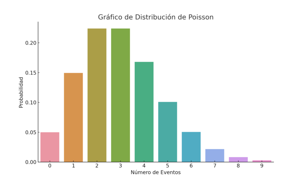
The Poisson distribution is ideal for modeling rare events in fixed intervals. Its sole parameter, λ (lambda), represents the expected number of occurrences in that interval.
- Collect historical demand data: count purchase orders per period.
- Determine λ: compute the historical rate. If you see 1 order every 45 days, the daily rate is
- $$r = \frac{1}{45}\approx0.0222\;\text{orders/day}$$.
- For a 60‑day horizon: $$λ60=r×60=1.333.$$
- Estimate probabilities: $$P(k) = \frac{\lambda^k e^{-\lambda}}{k!}$$
- Combine with observed lead time to forecast total replenishment time.
- Adjust safety stock based on the probability distribution to minimize stockouts.
For Example:
For a 60‑day period (λ = 1.333), the probabilities of k orders are:
| k | P(k) (approx.) |
|---|---|
| 0 | 26.3 % |
| 1 | 35.1 % |
| 2 | 23.4 % |
| 3 | 10.4 % |
| 4 | 3.5 % |
This allows us to achieve a probabilistic prediction of future demand in any desired period. I hope this clarifies how to apply Poisson in practice for lead time forecasting.
2. Prioritize with Pareto (ABC) analysis
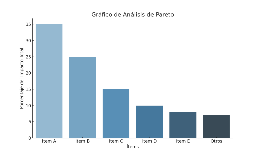
Comparing the Poisson distribution with other methods can be enlightening. For instance, Pareto analysis, based on the 80/20 principle, is useful for identifying the few critical components that may represent the majority of problems or costs in inventory management.
The 80/20 rule segments inventory by impact:
- A items (20 %): ~80 % of value or risk
- B items (30 %): ~15 %
- C items (50 %): ~ 5 %
By ranking SKUs by cost or criticality and plotting cumulative percentages, you focus resources on the “vital few.”
Advantages:
Simple to implement in spreadsheets
Allows focusing on truly critical SKUs
Guides inventory policy segmentation by importance
3. Quantify uncertainty with Jackknife

The Jackknife is a resampling technique introduced by Quenouille (1956) and popularized by Tukey (1958) that provides robust estimates of bias and variance for any estimator. It systematically leaves out one observation at a time (or one block) to evaluate the sensitivity of your results.
3. Quantify uncertainty with Jackknife (Expanded)
The Jackknife is a resampling technique introduced by Quenouille (1956) and popularized by Tukey (1958) that provides robust estimates of bias and variance for any estimator. It systematically leaves out one observation at a time (or one block) to evaluate the sensitivity of your results.
Mathematical formulation
Let $$(\hat\theta)$$ be an estimator computed on the full dataset of (N) observations. For each $$(i = 1, \dots, N)$$, define the leave‑one‑out estimate
Algorithmic steps
- Compute the estimator $$(\hat\theta)$$ on the full dataset.
- For each (i), remove the (i)th observation and recompute $$(\hat\theta_{(i)}).$$
- Calculate $$(\bar{\theta}_{(-\cdot)})$$, the average of all leave‑one‑out estimates.
- Use the formulas above to compute bias and variance estimates.
- Derive confidence intervals or adjust safety‑stock margins accordingly.
Practical considerations
- Computational cost: (O(N)) estimator evaluations. For very large (N), consider a block‑Jackknife (omit contiguous blocks instead of single points).
- Time‑series data: if observations are autocorrelated, remove blocks of consecutive points to preserve structure.
- Block size: experiment with different block lengths to balance bias and variance.
- Alternatives: the Bootstrap can yield more accurate confidence intervals for complex estimators.
By applying Jackknife, you gain a clear measure of uncertainty in your demand forecasts, strengthen confidence in your safety‑stock decisions, and detect potential outliers in your data.
Implementing Poisson, Pareto, and Jackknife together lets you:
- Predict demand probabilities aligned to your lead‑time window
- Prioritize high‑impact components in inventory planning
- Validate forecast robustness and set safety stocks with quantified confidence
Have you applied any of these methods? Share your experiences and results!